Looking beyond the independent electron approximations

1. Hartree Approximations
2. Hartree-Fock approximations
3. Hartree-Fock for the case of free electron gas
4. The origin of the Screening potential
5. Screening potential of the free electron gas
6. Two ways to calculate susceptibility
- 6.1. Thomas-Fermi method
- 6.2. Lindhard method
7. Resources

1. Hartree Approximations

If the force on a electron in the materials would not have dependent on the position of other electrons (i.e. all the electrons are independent of each other), then we can straight forward solve the schrondinger equations to find the wave functions (which describes the states, i.e. positions and velocity of the electrons): \[\frac{\hbar^{2}}{2m} \nabla^{2} \psi + U(r) \psi = E \psi.\] Here $\psi(r_{1}s_{1},r_{2}s_{2},r_{3}s_{3},...)$ is the wave functions of the electrons with states $\left( r_{1}s_{1} \right)$,$\left( r_{2}s_{2} \right)$, $\left( r_{3}s_{3} \right)$… Important to note that the electrons are independent to each other. The equation can be solved easily by solving the $N$ numbers of independent equations assuming the wave functions of the form $\psi(r_{1},s_{1})=A(r_{1},s_{1})\mathrm{e}^{\imath k r_{1}}u(s_{1})$.
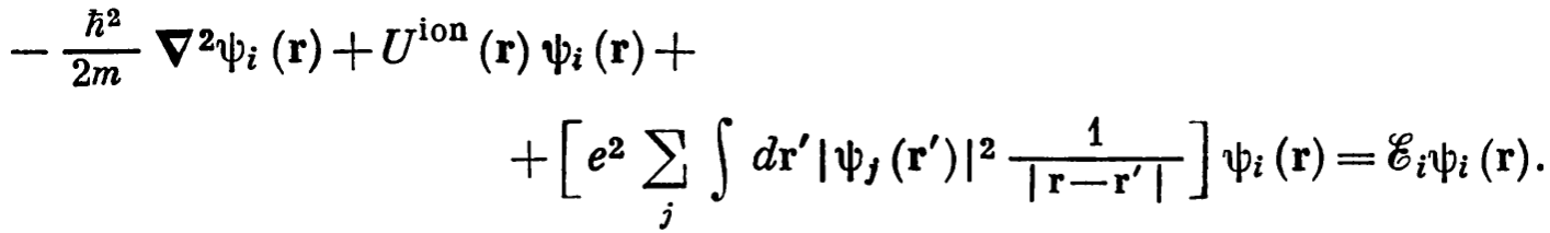
However in the real materials the electrons dependent on the position of the other electrons. The most general equations to solve in the materials is: Here $\Psi(r_{1}s_{1},r_{2}s_{2},r_{3}s_{3},...)$ is the wave function which depends on the position of the other wave function. First part is the Kinetic energy which calculates the energy of the electrons at $(r_{1},s_{1})$. The second part is the attractive potential energy of electrons at $(r_{1},s_{1})$ due to positively charged ions at positions $\mathbf{R}$. Third part is the repulsive interaction on the electrons at position $r_{1}$ due to electrons at all other positions $r_{j}$.
However it is very hard to solve this problem for large number of electron. As the set of equations are interrelated to each other. If we want to find the wave functions for $\psi\left( r_{1},s_{1} \right)$ we need to know the wave functions for all other wave functions $\psi\left( r_{2},s_{2} \right)$, $\psi\left( r_{3},s_{3} \right)$… This is impossible.
Therefore to solve this problem we first collect all the potential terms together: $U=U_{ion}+U_{el}$. And rewrite the Schrodinger equations as: \[\left( -\frac{\hbar^{2}}{2m} \nabla_{i}^{2}+U\right)\Psi= E \Psi.\] $U_{ion}$ is the periodic function with periodicity of the ions. And $U_{el}(r)=\frac{1}{2} \int\limits_{r'} \rho(r')/|r-r'|dr'$.
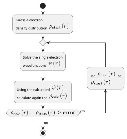
$U_{ion}$ is very easy to calclate, and interaction from all other electrons are taken into account through electron density functions $\rho(r)$. Now the our job is to solve the one body problem in an effective potential $U$. It is easier to solve. The complete Hartree Hamiltonian is:
Therefore following flow charts should be used

2. Hartree-Fock approximations

The Hartree-Fock approximation is different from Hartree approximation only by the inclusions of the interaction terms. In the Hartree method the change in the positions of the electrons in the wavefunctions does not make into antisymmetric – $Ψ(r₁,r₂) ≠ Ψ(r₂,r₁) $ – which should be as we are dealing with the fermions.

However, the Hartree-Fock method remedies this shortcoming by using slater determinants for the wave functions. All the other assumptions of the Hartree method are kept intact. Assuming the wave functions of the individual electrons as $\Psi(r_{1},r_{2},\dots)=\psi(r_{1})\psi(r_{2})\dots$ the slater determinant can be written as:

	r1	r2	r3	r4
elec-1	$\psi_{1}(r_1)$	$\psi_{1}(r_2)$	$\psi_{1}(r_3)$	$\psi_{1}(r_4)$
elec-2	$\psi_{2}(r_1)$	$\psi_{2}(r_2)$	$\psi_{2}(r_3)$	$\psi_{2}(r_4)$
elec-3	$\psi_{3}(r_1)$	$\psi_{3}(r_2)$	$\psi_{3}(r_3)$	$\psi_{3}(r_4)$
elec-4	$\psi_{4}(r_1)$	$\psi_{4}(r_2)$	$\psi_{4}(r_3)$	$\psi_{4}(r_4)$

Note that the rows represent the electrons, and the columns represent the positions in the slater determinant.

Using this wave functions one can find the Schordinger Equations as: 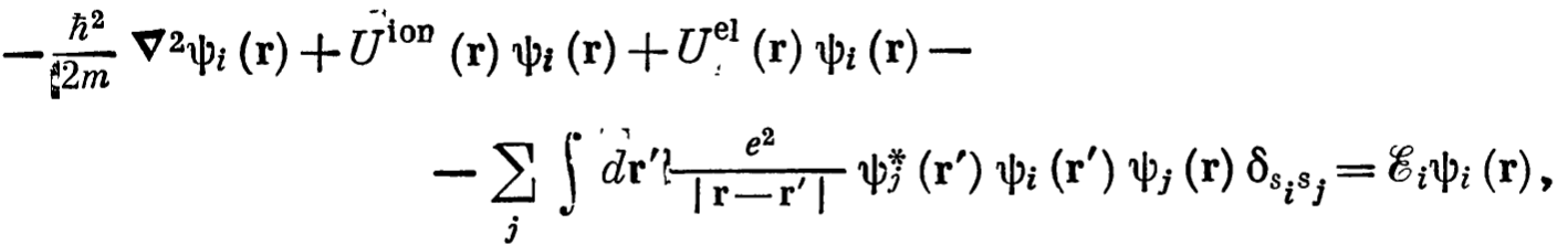The first part is the kinetic energy, the second is the attractive interaction due to ions (the sign of the potential is negative from the initial equations), the third part is the repulsive force between electrons, and 4 th part is the exchange interaction, which appears due to antisymmetric wave functions of the fermions. Regarding the signs:

Energy type	sign	Attractive	Operator
		or Repulsive
Kinetic Energy	Negative	N/A	$-\frac{\hbar^{2}}{2m} \nabla^{2}$
Ionic Potential	Negative	Attractive	$U_{\text{ion}}=-\sum\limits_{R}\frac{Ze^{2}}{r-R}$
Energy
Electric Potential	Positvie	Repulsive	$U_{\text{e-e}}=+ \sum\limits_{r'} \frac{e^{2}}{r-r'}$
Energy
Exchange potential	Negative	Attractive	$U_{\text{int},i}=-\sum\limits_{j} \int dr' \frac{e^{2}}{r-r'} \psi_{j}^{}(r') \psi_{i}^{}(r') \psi_{j}(r) \delta_{s_{1}s_{2}} \psi_{i}(r)$

Special attention should be played to the exchange potential. In simple words it calculates the sum of potential energy (repulsive) due to two situations:
- Repulsive potential at position $r'$ due to electron at position $r$.
- Repulsive potential at position $r$ due to electron at position $r'$.
- Moreover, the spin should be same at both $r$ and $r'$. Otherwise the potential is zero.
Besides the exchange potential is negative. It means the presence of exchange potential is profitable for the system.

3. Hartree-Fock for the case of free electron gas

In case of free electron gas previously we solved the Schrodinger equation (neglecting electron-electron correlations). However when electron-electron correlation is taken into account we need to add the exchange field in the Schrodinger equation.
To eigen functions will be plane wave with spinors: \[\psi_{i}(r) = \sum\limits_{k} e^{\imath k r} \begin{pmatrix} \psi_{s_{1}}\\ \psi_{s_{}{2}}\end{pmatrix}\].
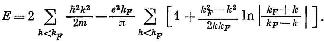
The total solution of the Hamiltonian will give the energy:
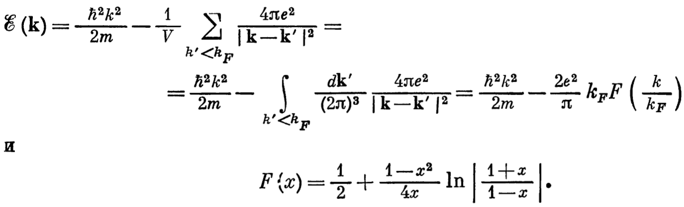
The first part is the usual kinetic energy with quasi momentum $\hbar k$. The second part is the correction due to electron-electron correlation. If compared to the energy for free electron gas without interaction we had only the first part. We also note that the energy now is smaller (second term is negative) than the free electron gas (without correction). The dependence of the electron electron correlation correction on the momentum (w.r.t $k_{f}$) is below:
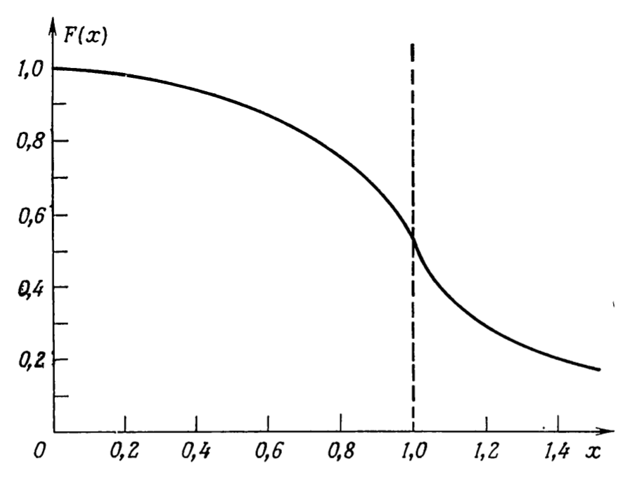
From the graph it shows that energy is negative when $k=0$ for correlation case ($\varepsilon(k=0)= 2 e^{2}/\pi k_{F}$), compared to no correlation case ($\varepsilon(k=0)=0$).
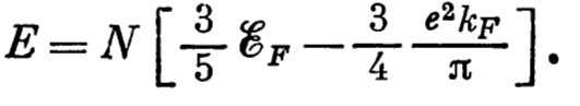
The total energy of the electron gas and density of energy are:
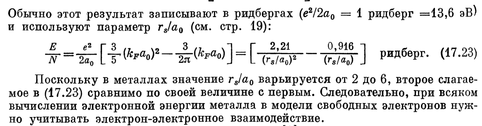
Slater in his work ( https://doi.org/10.1103/PhysRev.81.385, https://doi.org/10.1103/PhysRev.82.538, https://doi.org/10.1103/PhysRev.91.528) proposed to replace the total exchange potential in the full Schrodinger equation by the constant calculated as $\varepsilon^{\text{exchange}}=-0.916/(r_{s}/a_{0})$. In this case we need to solve just The Schrodinger equation with some constant.
At $k=k_{F}$ i.e. $x=1$ the function $F(x)$ and hence the energy $\varepsilon(k_{F})$ will be infinity. It also means the velocity $v = \frac{\partial \varepsilon}{\partial k}=\infty$. Which means the energy density at the Fermi levels is infinity. Which means the specific heat $c_{v}=\partial u/ \partial T$ is also infinity.

4. The origin of the Screening potential

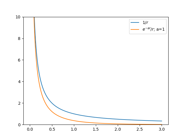
In the energy expression for free electron gas one can see that for exchange energy at $k=k_{F}$ the energy is $\infty$. It happens due to $1/k$ terms in the fourier expansion of the Coloumb potential. However instead of $F \propto 1/r$ coloumb potential we will take some modified coloumb potential of form $F \propto e^{-k_{0}r}/r$ then this $\infty$ does not appear. A comparison between two potential is given below
```
import numpy as np
import matplotlib.pyplot as plt
import sys

r=np.linspace(0.001,3,1000)
a=1
coloumb=1/r
mod_columb=np.exp(-a*r)/r

fig,ax=plt.subplots()
ax.plot(r,coloumb,label=r'$1/r$')
ax.plot(r,mod_columb,label=r'$e^{-ar}/r$; a=1')
ax.set_ylim(0,10)
ax.legend()
plt.savefig(sys.stdout.buffer)
```
Physically, we can defend the assumption of using the potential of type $e^{-ar}/r$ instead of $1/r$. If one takes the potential of type $1/r$ then the fourier transform will have the fourier coefficients $V(k) \propto e^{2}/k^{2}$; then when $k=0$ the Fourier coefficient becomes $\infty$. Physically it means the wave function corresponding to $k=0$ which is $e^{i k r}V(k) \approx V(k)$. Because the oscillating part ($e^{ikr}$) is almost constant. It means the effect of $V(k)$ is long. However, if we take the potential $e^{-akr}/r$ then the fourier coefficients become: $V(k) \propto e^{2}/\left( k^{2} + a^{2} \right)$. In this case at $k=0$ $V(k) = 1/a^2 \neq \infty$.
Physically the Fourier coefficients V(k) represent the radius applicability of the Coloumb potential. It can be understood by thinking that the $V(k) \approx 0$ as $k$ increases; it means only the oscillating part $e^{ikr}$ corresponding to low $k$ will give any values to the Coloumb potentials $V(r)$. If $V(k=0) \approx \infty$ then it means the V(k) corresponding to $k\approx 0$ will have higher values which will raise the base of the $V(r)$, which means for $V(r)$ to be zero large radius $r$ is needed. However if $V(k) \neq \infty$ for $k \approx 0$, then compared to the previous case the radius of the potential will be less. It can be clearly seen in above figure. It means the modified potential just decreases the long range radius of the Coloumb potentials.
As in the real material we don't see the breakdown of specific heat behaviour, we can say that when two electrons affects each other through exchange fields, other electrons in the materials arrange themselves in such a way that the protect the other electrons from feeling the full force of Coloumb repulsion. It is known as the Screening effects.

5. Screening potential of the free electron gas

When a positively charged ion is placed in the electron gas then negatively charged electrons around this ion creates a compensation potential. However the electrons which take part in creating this compensation potential also creates a potential which other electrons feels. These are called the screening potential.
Therefore there are three types of potential:
- $\phi_{\text{ext}}$ — External potential created by the positively charged ions
- $\phi_{\text{ind}}$ — Induced potential created by the electrons around ions
- $\phi$ — Resulting screening potential create by summation of the external and induced potential
The aim is to find the $\phi$. In analogy to the electromagnetic theory one can write the screening potential as the resulting potential due to external potential multiplied by the permitivity: \[\phi_{\text{ext}}(r)= \int\limits_{r'} \varepsilon(r,r') \phi(r').\] $\varepsilon(r,r')$ is the permitivity at $r$ due to total potential at φ(r'). For homogeneous gas the $\varepsilon(r,r')=\varepsilon(r-r')$. Therefore we will have: \[\phi_{\text{ext}}(r)= \int\limits_{r'} \varepsilon(r-r') \phi(r').\]
Usually in condensed matter the properties are analyzed in the frequency space, therefore taking the Fourier transform on both sides we will get: \[\phi_{\text{ext}}(k)= \varepsilon(k) \phi(k).\]
Usually we know the external potential $\phi_{\text{ext}}(k)$, therefore, we should know $\varepsilon(k)$ to find the $\phi(k)$.
It is better to work in the charge density when potential is involved. The potential is related to the charge density through Poisson equations. To find the $\phi(k)$ we will use the Possoin's equation: \[-\nabla \phi(r)=4 \pi\rho(r).\] The Fourier transform of above equation is: \[k^{2} \phi(k)=4 \pi\rho(k).\]
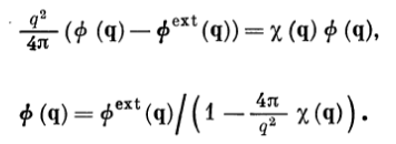
The idea is to compare equation $\phi_{\text{ext}}(k)= \varepsilon(k) \phi(k)$ with the analogous equation found from the equation: \[\rho^{\text{ind}}(q)=\chi(q)\phi(q).\] We will use $\rho_{\text{ext}}(k)=\rho(k)-\rho_{\text{ind}}(k)$ in above equations; we also use \[\rho(k)=\frac{k^{2}}{4 \pi} \phi(k).\] \[\rho_{\text{ext}}(k)=\frac{k^{2}}{4 \pi} \phi_{\text{ext}}(k).\] \[\rho_{\text{ind}}(k)=\frac{k^{2}}{4 \pi} \phi_{\text{ind}}(k).\]
Putting all these values we will get:

6. Two ways to calculate susceptibility

The main aim is to find the induced electronic density $\rho_{\text{ind}}$ or the susceptiblity $\chi$ for a given potential $\phi$.
Following two methods are used.

6.1. Thomas-Fermi method

The main idea of Thomas fermi is to assume that the energy dependence of electrons on wave vector $k$ and space $r$, can be written as: \[\varepsilon(k,r)= \frac{\hbar^{2}k^{2}}{2m}-e\phi(r).\] It is assumed that the above energy dispersion is found from the solution of the Schrodingers' equation with potential $\phi(r)$,i.e. \[-\frac{\hbar^{2}}{2m} \nabla^{2} \psi_{i}(r)-e\phi(r) \psi_{i}(r)=\varepsilon_{i}\psi_{i}(r).\]
If we know the energy dependence on $\varepsilon(k,r)$ then we can write the spatial dependence of chemical potential: \[n(k,r)=\frac{1}{\mathrm{e}^{\left( \varepsilon(k,r)-\mu \right)/k_{B}T}}\]
The density of electron at some points $r$ can be found by integrating $n(k,r)$ over all the $k$ values: \[\int\limits_{k} n(k,r) dk\]
In the absence of external potential the distribution $n(k,r)$ does not depend on the position $r$. Therefore we can write $n(k,r)|_{\phi_{ext}=0}\equiv n_{0}$.
In this case the induced potential can b written as $\rho_{ind}(r) = -e \left[ n(k,r)-n_{0} \right]$. Meaning the induced electon density only takes into account the extra electron density due to external charges.
In other words we can write: where
The main assumptions is following: we assume that in above equations $\phi(r) approx 0$. In this case we can Taylor expand $n_{0}[\mu+e\phi(r)]$
In other words we assume $\mu+e\phi(r)\equiv \mu'$. The Taylor expansion around $\mu$ is: \[n_{0}[\mu+e\phi(r)] = n_{0}[\mu'] \approx n_{0}(\mu) + \frac{\partial n_{0}(\mu')}{\partial \mu} \left( \mu'-\mu \right)= n_{0}(\mu) + \frac{\partial n_{0}(\mu)}{\partial \mu} (e \phi(r))\]
Putting this we will find the induced charge density
Comparing this with the general equation $\rho^{ind}(r)=\chi(r)\phi(r)$ we will find \[\chi(r)=-e^{2} \frac{\partial n_{0}}{\partial \mu}.\]
As $\theta(r)$ independent of $r$ we can write $\chi(r)=\chi(k)$.
Anyway it shows that the external potential is screened in the interatomic distance.

6.2. Lindhard method

In case of Lindhard method we find that the potential $\phi(r) \sim \frac{1}{r^{3}} \cos 2kr$ is oscillating. It is also known as Friedel oscillation or Rudderman-Kittel.
One of the intuitive explanation of the Friedel oscillations is the constructive and destructive interference of the waves of electron density created by the impurities in the homogeneous electron gas.
If the external potential depends on the time and oscillating then, we just add term corresponding to the frequency of $\hbar \omega$ to the denominator.

7. Resources

Notes on variational wave functions: resources/Chapter-17/variational.pdf
Links to publications of J C Slater about the effective exchange potentials.

	r1	r2	r3	r4
elec-1	\(\psi_{1}(r_1)\)	\(\psi_{1}(r_2)\)	\(\psi_{1}(r_3)\)	\(\psi_{1}(r_4)\)
elec-2	\(\psi_{2}(r_1)\)	\(\psi_{2}(r_2)\)	\(\psi_{2}(r_3)\)	\(\psi_{2}(r_4)\)
elec-3	\(\psi_{3}(r_1)\)	\(\psi_{3}(r_2)\)	\(\psi_{3}(r_3)\)	\(\psi_{3}(r_4)\)
elec-4	\(\psi_{4}(r_1)\)	\(\psi_{4}(r_2)\)	\(\psi_{4}(r_3)\)	\(\psi_{4}(r_4)\)