Sommerfeld's twist to Drude's model
Table of Contents
- 1. Two types of models of metals
- 2. Application of the Fermi-Dirac distribution to the Free electron models
- 3. Digressed topics
- 4. Solutions
1. Two types of models of metals
- Sommerfeld model is just the redressed Drude model with the Fermi-Dirac distribution. Drude used the Maxwell-Boltzmann distribution for his works. In a simple sense the Maxwell-Boltzmann says that all the electrons will have zero energy, and hence, the electron gas freezes at T=0. However, the Fermi-Dirac distribution gives a cut-off energy. The electron will have non-zero velocity in this case.
- Sommerfeld's idea will be applied two types of physical model used for metals:
- The Jellium model
- The Free electron models
- The Free electron model is where the interaction (collision) between electrons, and electron ions are completely neglected. It is the same as the electrons are confined in a small box.
- The Jellium model is the same as the free electron model. However, the effect of the ions are added in this case through periodic background potential generated by the ions.
2. Application of the Fermi-Dirac distribution to the Free electron models
2.1. The wave vector as quantum number
In accordance with the assumption of the Free electron models, the non interacting electrons are confined in a box — physically it represent the confinement of the electrons inside the materials due to attractive force of the ions. To find the states of the electron one usually solves the Schrodinger equations with the cyclic boundary condition. The resulting wave function of the electrons can be represented as:
\begin{eqnarray} \label{eq:1} & \psi = \frac{1}{ \sqrt{V} } \mathrm{e}^{i \mathrm{k}r}. \end{eqnarray}- Here, \(k\) represent the crystal momentum of the electrons. It is also known as wave vector. \(k\) defines the energy of the states with \(\hbar^{2}k^{2}\). Due to cyclic boundary conditions it takes the discrete values \(k = 2 n\pi/L\), where \(n \in \mathsf{Z}\). Physically it means the electron with the least energy will have \(2\pi\) phase change from one end of the system to the other end. The next energy level of the electron will have \(4\pi\) phase changes. Hence, in the box will live electrons whose wave function will have phase change from one end to the other will be multiples of \(2\pi\). It is shown in figure: resources/Chapter-2/scan 23-09-01 17-30-47.pdf
- The question arises why the periodic boundary condition was taken, as the physical system is not periodic. Although, it is true, however the reason for taking periodic boundary condition is also motivated from the physical consideration. It sounds unusual, however one can explain as follows. In the bulk the electrons are always moving, this can best be represented by the moving electronic wave function. If one does not take the periodic boundary condition — meaning the wave function becomes zero at the start and end of the confined box \(\psi(0)=\psi(L)=0\) — then the solution of the wave function will be a standing wave. It means the electron is not moving, which is not correct from the physical point of view.
2.2. Properties of the wave vector \(k\)
The importance of the wave vector:
The wave vector plays the central role in the analysis in the condensed matter physics, as every wave vector represent a single state \(k\) with energy \(\hbar^{2}k^{2}/2m\). This is because of the statistical physics, which relates the properties of the materials to some fundamental and general quantities like free energy, chemical potential. The Free energy, Chemical potential all depend on the energy occupied by the electrons of the material, which depends on the wave vector \(k\).
Density of states in momentum space: The momentum space is analogous to the three dimensional \(x, y, z\) space defined by axes \(k_{x},k_{y},k_{z}\). In this space every state occupies a volume of \((2\pi/L)^{3}\). To understand this one need to think momentum space as the continuous space, then one need to consider the fact that, the momentum can take the quantized values \(k=2\pi n/L\). In this case, there wont be any available states in between two adjacent \(k\) values, \(k=2 \pi n/L\) and \(k = 2 \pi (n+1)/L\). Hence every energy states contains the volume \((2 \pi/L)^{3}\). For example in a wire of 1 cm long there will be \(10^{8}\) atoms, and if every atoms will give one electron then in this wire we will have \(10^{8}\) electrons. If every electron represent a single energy states \(k\), then the momentum space will have minimum of \(10^{8}\) points along the direction along the \(k_{x}\) axis. As the value \(10^{8}\) is very large in the momentum space, hence, the \(k\) points are very close each other. This allow us to treat the momentum space as the continuum.
In the view of the author the mentioned reason in the book for treating the momentum space as continium, i.e. large $L$ gives very densed $k$-space is somewhat misleading. The main reason is the presence of the very large amount of electronic states.
In this continum limit, any volume \(\Omega\) in momentum space will contain \(\Omega/\left( 2 \pi /L^{3} \right)\) states.
- Fermi Momentum:
It is the highest value of \(k_{F}\) which is possible in the material. If given Fermi momentum one can find different other thermodynamic properties of the material.
No. of states in the systems: If the system is a usual box without any external force, then the occupied states create a sphere. The volume of the sphere will be \(4 \pi k_{F}^{3}/3\). As every state have the volume \(\left( 2 \pi/L \right)^{3}\), then the number of particles will be:
\begin{eqnarray} \label{eq:2} N = 2 \frac{4 \pi k_{F}^{3}}{3} \frac{V}{8 \pi^{3}} = \frac{k_{F}^{3}V}{3 \pi^{2}}. \end{eqnarray}- Density of states is \(n=\frac{k_{F}^{3}}{3 \pi^{2}}\). It is a very important parameter, as it connects the physically observable conductivity of the materials and density of electronic states, which in turn relates to the Fermi momentum. Conductivity is related to the current density as \(J = \sigma E\). Current density is the amount of unit charge flowing through an unit area in a unit time. In the Drude model \(\sigma = ne\tau/m\). One can substitute for \(n\) is this equation.
- Fermi velocity \(v_{F} = \hbar k_{F}/m\)
- Fermi Temperature \(T_{F} = \varepsilon_{F}/k_{B}\)
- Properties of Free Electron Gas In the Jellium model as we have assumed that electrons are confined to the box. Usually one can calculate the properties of this gas by applying usual statistical physics methods, for pressure, Bulk moduli.
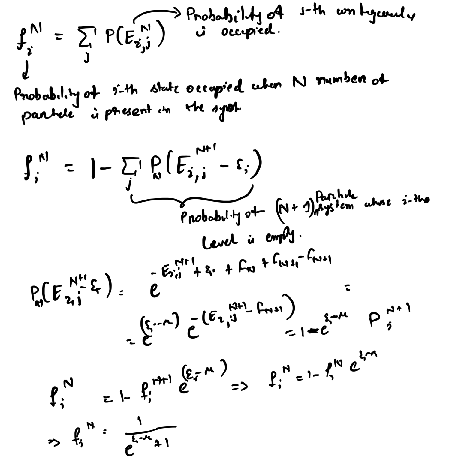
2.3. Derivation of Fermi Distribution ATTACH
- The main idea in the picture:
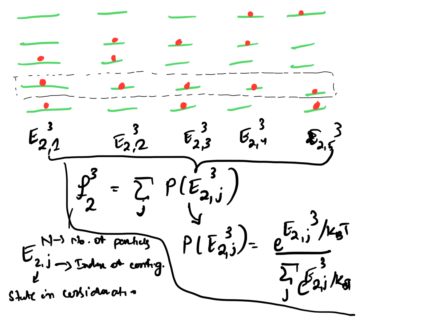 .
. - The derivation:
2.4. The specific-heat of the metals using the Fermi-Dirac distribtions
2.4.1. The difference between specific heat and chemical potential
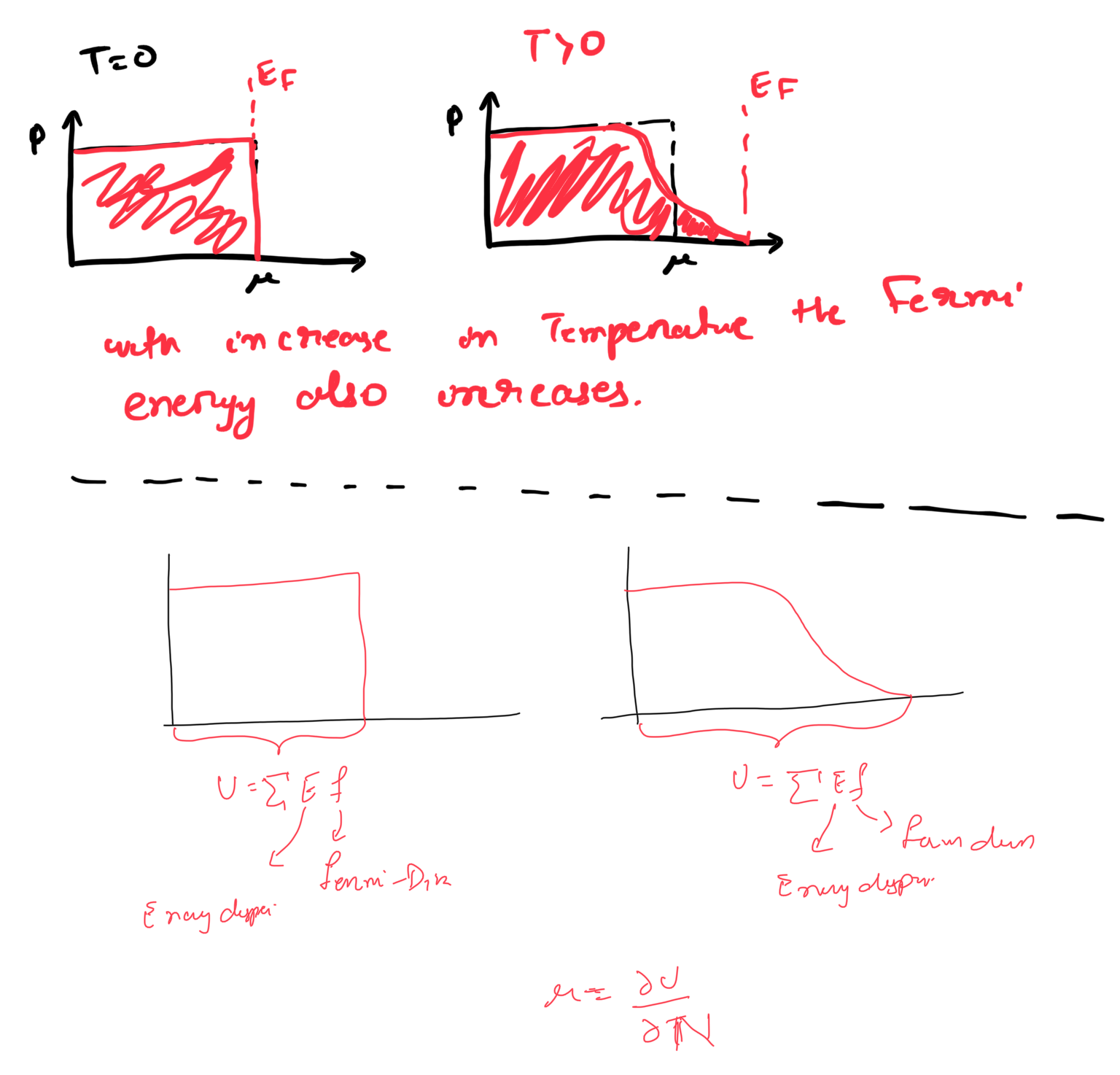
- The chemical potential is the amount of energy required to add a single particle to the system, while the volume is kept constant [see Eq. 24.6 of cite:&landau-05CoursesTheoretical-2005] \[\mu = \left( \frac{\partial U}{\partial N} \right)_{N}\] The Fermi energy is defined as the highest occupied energy of the system.
- With the increase in temperature usually higher energy states are occupied. This provides means the Fermi Energy is increased with temperature.
- The chemical potential takes into account the total energy of the system. One finds the total energy by multiplying the energy dispersion with the Fermi-Dirac distribution. In this sense the total energy of the system changes with increase in temperature as the contribution from the higher states, which were not occupied at \(T=0\) will also come into play.
- Hence, with increase in temperature both \(\mu\) and \(E_{F}\) changes, but the change in \(E_{F}\) is larger than the change in chemical potential \(\mu\).
- Some good answer to the questions:
2.4.2. Difference between temperature and Fermi temperature
- Fermi temperature is the temperature equivalent of the Fermi energy. it is found by the relation: \[E_{F}=k_{B}T_{F}\]. Here, \(K_{B}\) is the Boltzmann constant.
- Boltzmann constant physically related to the energy associated with a microscopic degree of freedom of a macroscopic system at non-zero temperature. Every microscopic state has energy \(1/2 k_{B}T\). That is why an atom with three degrees of freedom will have total energy of \(3/2 k_{B}T\). To every \(1/2 k_{B}T\) corresponds to the 0.013 eV.
- Although to every electron very small energy \(\hbar^{2}k^{2}\), as the Planck's constant \(\hbar=6.582 \times 10^{-16}\) eV, is very small. However, due to summation over Avogrado's number of electron the total energy becomes very big.
- In nonzero temperature only the electrons on the surface of the Fermi surface gets affected, specifically upto the depth of \(k_{B}T\) from the Fermi surface. The electrons which are very deep in the Fermi sea dont get affected, as there the energy acquired by the electrons is not sufficient to elivate them to the non occupied states.
- Hence, room temperature and zero temperature electronic configurations are very close to each other.
2.4.3. Sommerfeld Expansion
- The Sommerfeld Expansion relates the properties of the system at zero temperature and non-zero temperature. It is based on the assumption: at non-zero temperature only electrons which are near the Fermi surface participates in deciding the energy of the system.
- In other words the non-zero temperature property is just a peturbation of the zero-temperature property of the system.
- The summation of the property over the full energy can be written as: \[H(\epsilon) f(\epsilon) d \epsilon = \int^{\mu} H(\epsilon) d \epsilon + O(T^{2}).\] The first term represents the value corresponding to the zero temperature. However the second terms onward represents the higher powers of the temperature.
- With this idea it can be shown that the chemical potential varies from its zero temperature values by second order.
- The second order temperature difference can be understood physically. When the temperature is non-zero \(\mathcal{O}(k_{B}T)\) amount of electrons are excited, besides, these electrons have the \(\mathcal{O}(k_{B}T)\) of energy. Hence, the any property differs from its zero temperature value by second order in temperature.
2.4.4. Specific Heat of electrons
- The specific heat of electrons can be found as the differentiation of the Free energy with respect to the temperature. Physically how much energy is added to the system with unit change in the temperature: \[c_{v} = \frac{\partial U}{\partial T} = \frac{\pi^{2}}{2} \frac{k_{B}T}{E_{F}}nk_{B}.\]
- If we compare this term with classical — free electron gas -— specific heat \(c_{v} = \frac{3}{2} nk_{B}\), then comparing, we will find that the effect of temperature is to decrease the electronic contribution by \(\pi^{2}/3 k_{B}T/E_{F}\).
- From experiment specific heat is calculated from the following method. Specific heat has two contribution electronic and ionic. Electronic specific heat changes as \(c_{v}^{e} = \gamma T\), and ionic specific heat changes as \(c_{v}^{ionic} = A T^{3}\). Hence, electronic specific heat changes linearly with temperature, and ionic specific heat changes as cube of temperature.
- To find \(\gamma\), one calculates the total specific heat in experiment: \(c_{v} = c_{v}^{e} + c_{v}^{ionic}\), then divides this total specific heat by the temperature to get: \[\frac{c_{v}}{T} = \gamma + A T^{2}.\] From above equation if we plot \(c_{v}/T\), then the x-ordinate crossing of the specific heat will give the electronic contribution of the specific heats.
3. Digressed topics
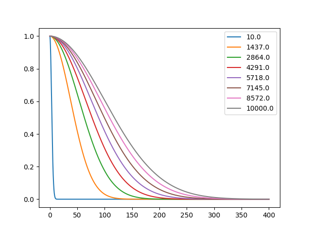
3.1. Maxwell-Boltzmann Distribution
  import numpy as np
  import matplotlib.pyplot as plt

  v= np.linspace(0, 400, 100000)
  T= np.floor(np.linspace(10, 10000, 8))
  max_botz= np.zeros((np.shape(T)[0],np.shape(v)[0]))
  for i,t in enumerate(T):
      # max_botz[i]= (1/(2*np.pi*t))**(1.5)*np.exp(-v**2/(2*t))
p      max_botz[i]= np.exp(-v**2/(2*t))

  fig, ax= plt.subplots()
  for i in enumerate(T):
      ax.plot(v, max_botz[i[0]], label=i[1])
  ax.legend()
  fname='resources/Chapter-2/Maxwell-Boltzmann.png'
  plt.savefig(fname)
  fname
  # plt.show()
4. Solutions
- Problem-1

- Problem-2

- Problem-2