The achievements and Fallacy of the Drude's model
Table of Contents
1. The History and Basic ideas
The model was proposed by the Drude in 1900. It was based on a simple idea: applying kinetic gas theory to the free electron gas. It was assumed that the valence electrons in materials form a non-interacting gas and they are confined in the volume of the materials. Their properties are controlled by the kinetic gas theory.
2. Assumptions
The Drude model is based on the four assumptions:
- Free and independent electrons
- Free electron alludes to the fact that electrons are not affected by the positive potential created by the ions.
- Independent electrons alludes to the fact that the interaction between electrons in the gas is completely neglected.
- In between collisions the electrons are affected only due to externally applied field through usual classical mechanics forces. For example under magnetic field the Lorentz force \(F_{L} \propto e v \times B\) acts on the electrons. The effect of ions or other electrons are completely neglected.
- Electron-Ion collision is the dominating mechanism
- The electron-electron collision can be completely neglected due to the fact that as electrons are of same nature then before and after collision the whole process appears as nothing has changed. See for example in following figure. resources/Chapter-1/scan 23-07-21 15-08-23.pdf
- On the Other hand the electron-ion collision does not look same as the ions are much heavier than electrons. resources/Chapter-1/scan 23-07-21 15-23-53.pdf
- Relaxation time
- It is defined as the average time between two collision process, and is represented as \(\tau\). The probability of the collision in time \(dt\) is \(dt/\tau\). If \(dt> \tau\) then the probability is always unity.
- In this approximation the relaxation time contains all the necessary information required regarding the collision process. In other words the microscopic details of the position of the electron, the collision process is not that important.
- Electron takes the local values after the collision
- After the collision process the properties of the electrons are completely controlled by the local values where the electrons gets collided. For example the kinetic energy of the electron will be higher if the electron gets collided in the regions where the temperature is higher compared to others.
3. Testing of the Drude assumptions through physical experiments
The Drude model gave the physical picture of the electronic process inside the materials. The assumptions made before explains how the electrons behaves inside the materials. However, to check whether the assumptions are correct or not, one needs to make experiments, find required values, and compare them with the assumptions made.
3.1. Conductivity
- The conductivity of electrons using Drude's assumptions can be represented as \[\sigma= \frac{n e^{2} \tau}{m} \implies \tau = \frac{m}{\rho n e^{2}}\]. Hence, the idea is to first measure the resistivity (1/conductivity). The value of \(n\) — density of electrons — is known from the Drude's argument, that every atom donates their valence electrons. The value of \(e\) — charge of electron in Coulomb \(1.6 \times 10^{-19} \: C\) is known. Using these values and experimental resistivity we find the relaxation time \(\tau\).
- Using the calculated value of \(\tau\) and average velocity of electron from kinetic theory of gas \(v\) we calculate the average distance travelled by electrons in between two collisions: \(l = v \tau\). If the value of \(l\) is reasonable then the assumption is correct. The velocity of electron in kinetic theory of gas depends on the temperature through \[\frac{1}{2}m v^{2}=\frac{3}{2} k_{B}T \implies v \frac{3 k_{B}T}{m}\].
- The values of \(\rho\) from the resistivity experiments is shown in Tab. 1.3 of cite:ashcroft-SolidStatePhysics-1976a. From these values one will find that \(l \propto 1-10\) Å. It is comparable to the inter ionic site distances.
- However, there are couple of errors in the above calculations due to classical treatment of electronic gas. The usual value of the velocity when treated quantum mechanically — meaning using Fermi distribution — one gets velocity two orders of larger than we found in classical treatments. Hence, at low temperature — where the \(\tau\) is order of magnitude larger — one would expect the relaxation path \(l\) to be of order \(l \propto 10^{3} --- 10^{4}\) Å. However, in the more carefully made measurements the experimental values of the \(l \propto 10^{8}\) Å. Hence, the Drude model is missing something in the collision process, and the \(\tau\) given through conductivity experiments and Drude's approximation is not the correct values.
- Due to this, relaxation time found from the Drudes' model is not a reliable metric. Hence, other quantities which don't depend on the relaxation time can be used to validate the Drudes' model.
- One of the idea here is to find the physical quantities which depend on the ratio of two quantities proportional to the relaxation time. For example if \(A \propto \tau^{n}\) and \(B \propto \tau^{n}\), then the ratio of the \(A/B\) will not depend on the relaxation time. Below we discuss the Hall conductivity relating to this idea.
- Another idea is to find the quantity which is multiplied or divided by the \(\tau\), i.e \(\tau/A\) or \(\tau \times B\). If \(A \gg \tau\) or \(A \ll \tau\), then \(\tau/A \sim 0\) and \(\tau/A \sim \infty\) respectively. In this case the whole quantity have almost constant value, and in effect the value of \(\tau\) is neglected. The plasma frequency found from the Drude model is one of this type of quantity.
- Another idea is to replace \(v\tau=l\) whenever it appears in the equation.
3.2. Hall coefficient
- In Hall experiments two types of measurements are done: (i) magneto resistance, (ii) hall coefficient. Magneto resistance is the resistance of the systems along the applied electric field. Hall coefficient relates the resistance along the perpendicular direction of the applied electric field. If electric field is along $x$-axis and magnetic field is along $z$-axis, then the Magneto resistance is $ρ (H)=Ex/jx $. For the same condition the Hall coefficient is \(R_{H} = E_{y}/j_{x}H\). It is found from the physical argument that the developed electric field along the perpendicular $y$-axis will depend on the applied magnetic field and the applied current along $x$-direction, i.e. \(E_{y} \propto j_{x} H_{z} \implies E_{y} = R_{H} j_{x} H_{z}\).
- The Hall coefficient predicted by the Drude model is defined as \(R_{H}=-1/nec\). It takes into account only the density of free electorns in the material. However, this conclusion is unphysical as one expect the dependency of the \(R_{H}\) on applied magnetic field and temperature. Hence, Drude model don't give the correct Hall coefficient. However, it gives the limiting values for the Hall coefficients for very low temperature and carefully prepared samples.
- All in all Drude model fails in the usual case to find the Hall coefficient.
3.3. Plasma frequencies
- Plasma frequency is related to the oscillation of electronic gas as a whole inside the material in equilibrium. When an electric field is applied to the materials, the electric field can be detected on the other side if the frequency of the applied electric field is larger than the plasma frequencies. From Maxwell's equation and complex conductivity found from the Drude model it is defined as \[\omega_{p} = \frac{4\pi n e^{2} }{m}\].
- One usually know the electron density of atoms \(n\), using these one can find the \(\omega_{p}\). The experiment has good agreement with alkali metals, but for other materials it fails. The alkali metals has a single electron in the outer \(ns^{1}\) shell. Hence it has single free electrons. The interaction can be neglected. Hence, it has good agreement with the experiments.
- One way of thinking of the presence of the plasma frequency is that, the electron gas oscillates with its own frequencies in equilibrium. If the applied frequency is more than the plasma frequencies then from the point of view of the applied frequency the electronic medium seems to be constant. However, if the applied frequency is smaller than the plasma frequencies, then from the point of view of the applied field, the electronic medium seems to be changing constantly.
- In this regard the Drude model fails to correctly find the Plasma frequencies.
3.4. TODO Wiedmann-Franz law
- Wiedmann-Franz law states that the ratio of the thermal conductivity to the electric conductivity is proportional to the temperature: \(\chi/\sigma \propto T\).
- Using Drude's assumptions it was found that \[\frac{\chi}{\sigma T} \propto \frac{3}{2} \left( \frac{k_{B}}{e} \right)^{2}\].
4. Digressed topics
4.1. Change in momentum of electron between two collisons
- Some physical things should be remembered. In equilibrium the total momentum of electron gas and the ion at any time will be zero, this is due to the fact that the current in equilibrium will be zero. Hence, \[p(t) = \sum\limits_{i} p_{i} (t) \equiv 0\]. Here, \(i\) is summed over all electrons and ions. Following process takes place in this picture:
- first at \(t=0\) electron approaches to an ion with momentum some momentum \(p(-\tau)\)
- Collides with the ion and gives its momentum to the ion — now the ion has opposite momentum \(-p(-\tau)\). However, electron takes the ion's momentum \(p(0)\).
- It travels a time \(\tau\)
- Gets again collided with some other ion, and transfers the momentum \(p(0)\) — as before the ion has the opposite momentum \(-p(0)\). As before electron takes the new momentum from the collided ion \(p(\tau)\).
- If considered the final ion then the change in momentum of that ion should have \(-p(0)\) after collision. If taking the system as two ions then their total momentum will always be zero \(p(0)+p(\tau)=0\). Change in momentum can be written as \(dp(t) = -p(0)\). One should always think in terms of the second ion when analyzing this situation
- One can introduce the probability in this case: \[dp = -p(0) \frac{dt}{\tau}.\] It says that the probability of the change in momentum of the second ion in time \(dp\) is \(-p(0) dt/\tau\).
- If some force is applied, then during traveling the electron will acquire the momentum \(dp = f dt\). Adding the two cases we will get the total change in momentum under the applied force will be: \[dp(\tau) = - p(0) \frac{dt}{\tau} + f dt.\]
4.2. Complex conductivity
When an electric field varying in time is applied to the material, the conductivity acquires the real and imaginary part \(\sigma(\omega) = \frac{\sigma_{0}}{1-i \omega \tau}\). Here, \(\sigma_{0}\) is the conductivity when a DC current is applied. The real part of the conductivity shows the conductivity of the electrons through dissipation. However, the imaginary part of the conductivity show the lossless part of the electron. The real and imaginary part of conductivity is shown below.
import numpy as np
import matplotlib.pyplot as plt
from math import *
x = np.arange(-10,10,1)
a = 1
y = a/(1-1j*x)
fig, ax = plt.subplots(2,2)
imag=ax[0,0].plot(x,np.imag(y))
ax[0,0].set_title('imaginary')
imag=ax[0,1].plot(x,np.real(y))
ax[0,1].set_title('real')
imag=ax[1,0].plot(x,np.abs(y))
ax[1,0].set_title('absolute')
fname='resources/Chapter-1/conduct-complex.png'
plt.savefig(fname)
fname
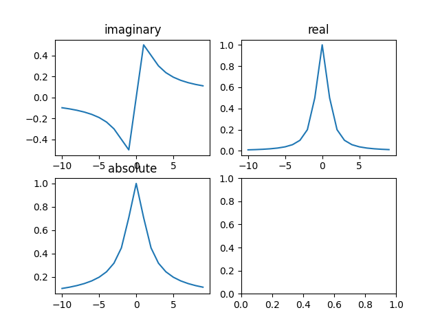
- If the applied field has high frequencies the conductivity decreases \(\propto \omega^{-1}\), then the free electrons can not travel required distance to get collided. Hence, the conductivity in that case becomes zero. The electrons in real space oscillates periodically without traveling large distances.
- The real and imaginary part of the conductivity appears due to inability of the electron gas to react instantly. When an electric field is applied along one direction the electronic gas travels in that direction. When the direction of the electric field changes the electron gas travels in the other direction. However, to change the direction of the electron gas first electron gas losses all its motion along the previous direction. Then starts to move in the opposite direction. This lag is represented in terms of the imaginary value.
- Another way of thinking about imaginary conductivity is from equation \(J(\omega)=\sigma(\omega)E(\omega)\). For DC field the current will be in phase with the field. It means the amplitude of the current will be proportional to the amplitude of the electric field at a given time. However, if an AC field will be applied then the amplitude of the current will lag the amplitude of the applied electric field. This lag is captured in the conductivity \(\sigma(\omega)\).resources/Chapter-1/scan 23-07-26 14-29-09.pdf
4.3. Polarization of the Electric field ATTACH
5. Solutions
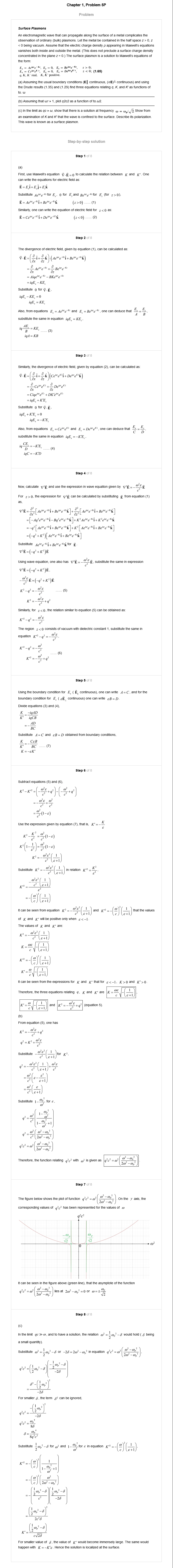
- Solutions to Problem-1
- Solutions to Problem-2
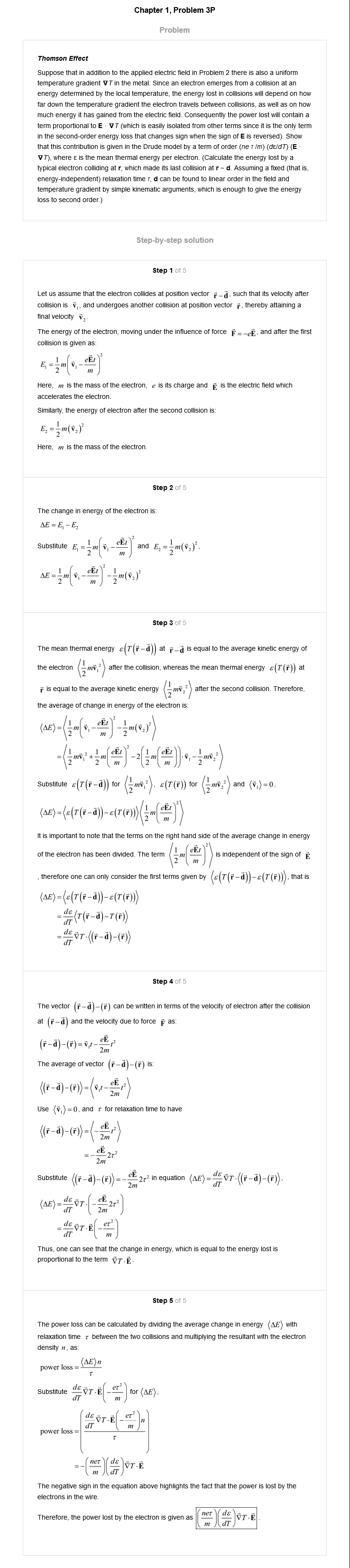
- Solutions to Problem-3
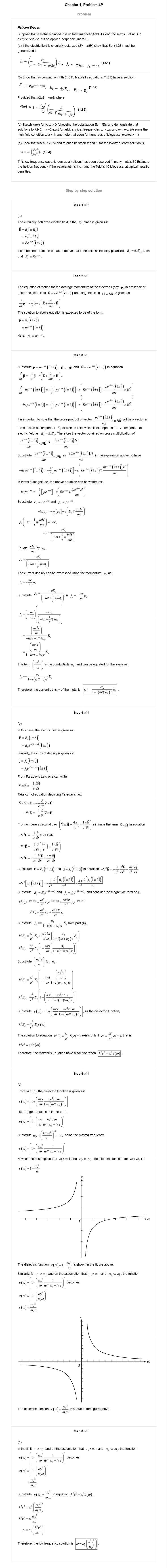
- Solutions to Problem-4
- Solutions to Problem-5